Are you like me where you come across incredibly specific problems with ecological data that nobody seems to be talking about despite it seeming like it should be common? If you are, then stick around because you might like this!
The Problem
So, the issue we’re trying to solve is this: ecologists (me) often collect categorical measurements for aspect (Like, is the side of the hill face North or Southeast?). This makes a lot of sense and is often useful and easy for simpler analyses like an ANOVA or T-tests. However, I have been fixated on trying to use the environmental similarity of different plots to explain how similar the plant communities are. That is where this method has broken down. Attempting to dummy variable each direction fails at capturing the fact that a plot facing Northwest is more similar to one facing North than one facing Southeast. When a good calculation of dissimilarity is at stake, that similarity needs to be accounted for!
I am well aware of the fact that I may be the only person to ever care about this. BUT, on the off chance that someone is searching for the answer to this very pedantic question, I thought it was worth putting out in the world. If you are here because you are seeking answers to this small but beguiling question (that really feels like someone else should have answered before!), I got you!
Here is my thought process and the answer is at the bottom! (Spoiler: the answer is actual math…)
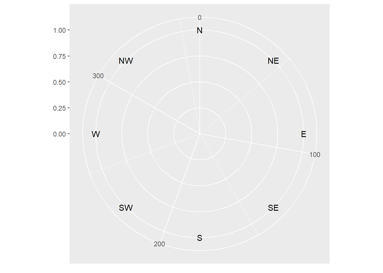
Okay, what you see above is a compass. I will be displaying the dissimilarity to North and Northeast for each direction here. The longer the line, the less similar, the smaller the more similar. We have a couple of requirements:
The opposite direction has to be the most dissimilar
The closest directions have to be the least dissimilar
The in-between directions have to increase at the same rate clockwise and counter-clockwise
The shapes have to preserved just rotated when comparing to North and Northeast
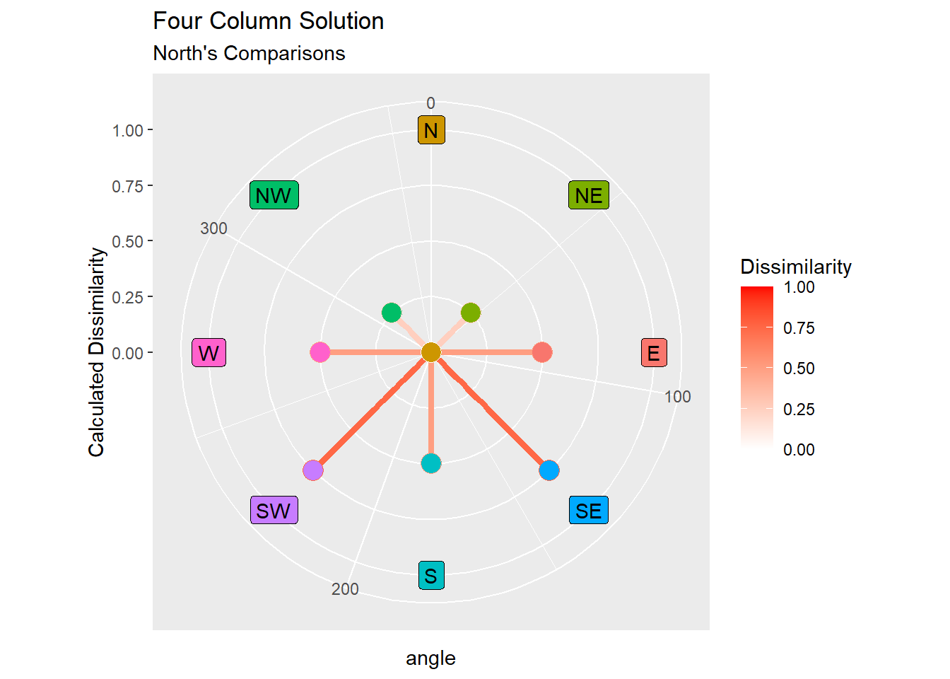
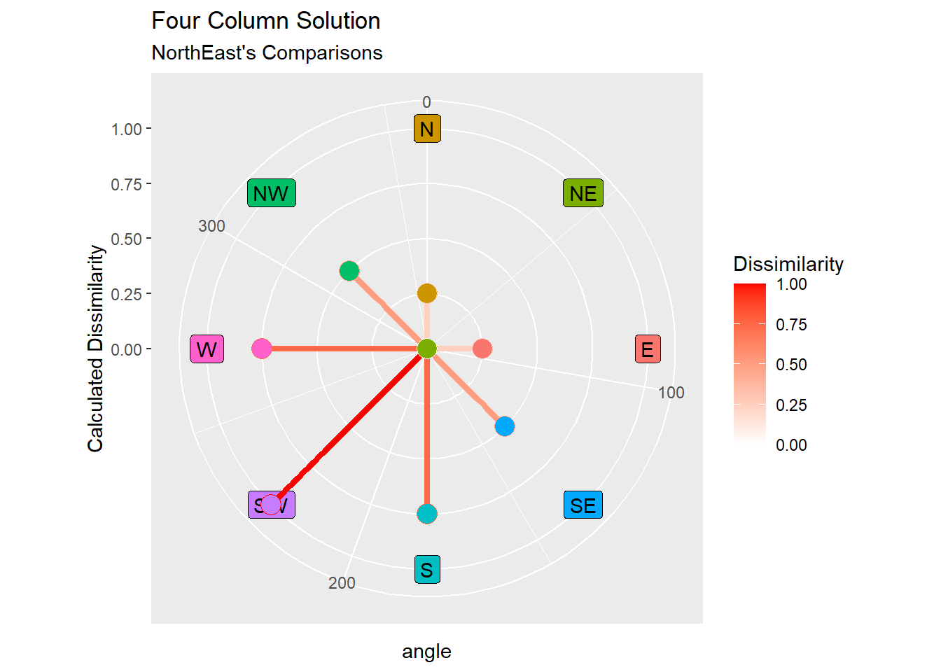
Four Column Solution
I really thought this was just going to work. I first tried a ‘four column solution’ where I categoized each direction by whether they included N,S,W, and E. For example, ‘North’ got a 1 in the north column whereas ‘Northeast’ got a 1 for the north and east columns.
FourCol <-data.frame(row.names =c("N", "NE", "E", "SE", "S", "SW","W","NW"), N =c(1,1,0,0,0,0,0,1), S =c(0,0,0,1,1,1,0,0), W =c(0,0,0,0,0,1,1,1), E =c(0,1,1,1,0,0,0,0))FourCol
   N S W E
N  1 0 0 0
NE 1 0 0 1
E  0 0 0 1
SE 0 1 0 1
S  0 1 0 0
SW 0 1 1 0
W  0 0 1 0
NW 1 0 1 0
It seemed so simple! So I used gower’s dissimilarity (I tried others) to see how the dissimillarities would shake out. I summed them for all directions with the assumption that they should all add up to be the same and, well….
  N  NE   E  SE   S  SW   W  NW
3.5 4.0 3.5 4.0 3.5 4.0 3.5 4.0
Uh, oh!!! Here are some plots demonstrating this issue!
FourDisNorth<-cbind(plotsetup, dissim =as.matrix(FourDis)[,1])FourDisNE<-cbind(plotsetup, dissim =as.matrix(FourDis)[,2])ggplot(data = FourDisNorth, aes(x = angle, y = dissim, color = dissim, fill = direction))+coord_polar(clip ="off")+scale_x_continuous(limits =c(0,360))+scale_y_continuous(limits =c(0,1))+geom_label(aes(label = direction, x = angle, y =1), color ="black")+geom_segment(aes(y =0, yend = dissim), linewidth =1.5)+geom_point(size=5, shape =21)+scale_color_gradient2( high="red", limits =c(0, 1), name ="Dissimilarity")+labs(title ="Four Column Solution", subtitle ="North's Comparisons", y ="Calculated Dissimilarity")+scale_fill_discrete(guide ="none")
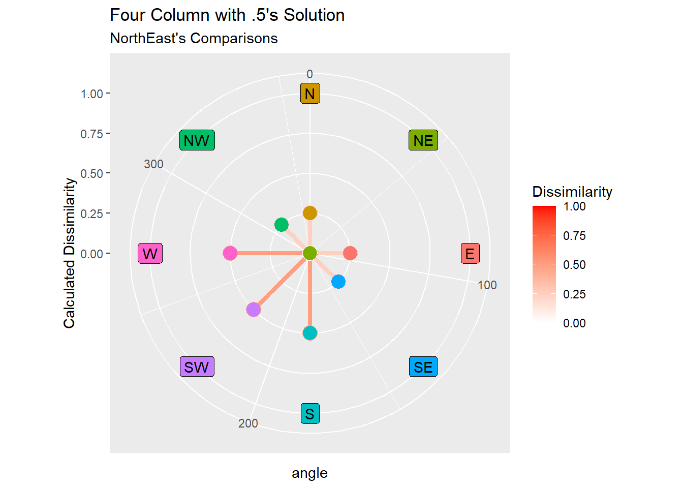
ggplot(data = FourDisNE, aes(x = angle, y = dissim, color = dissim, fill = direction))+coord_polar(clip ="off")+scale_x_continuous(limits =c(0,360))+scale_y_continuous(limits =c(0,1))+geom_label(aes(label = direction, x = angle, y =1), color ="black")+geom_segment(aes(y =0, yend = dissim), linewidth =1.5)+geom_point(size=5, shape =21)+scale_color_gradient2( high="red", limits =c(0, 1), name ="Dissimilarity")+labs(title ="Four Column Solution", subtitle ="NorthEast's Comparisons", y ="Calculated Dissimilarity")+scale_fill_discrete(guide ="none")
Well, a handful of issues immediately jump out. First, North and South are not the most dissimilar in North’s plot. Interstingly Northeast is most dissimilar to Southwest in the second plot. But, they don’t preserve the shapes between them! I want North’s plot to look like Northeasts!
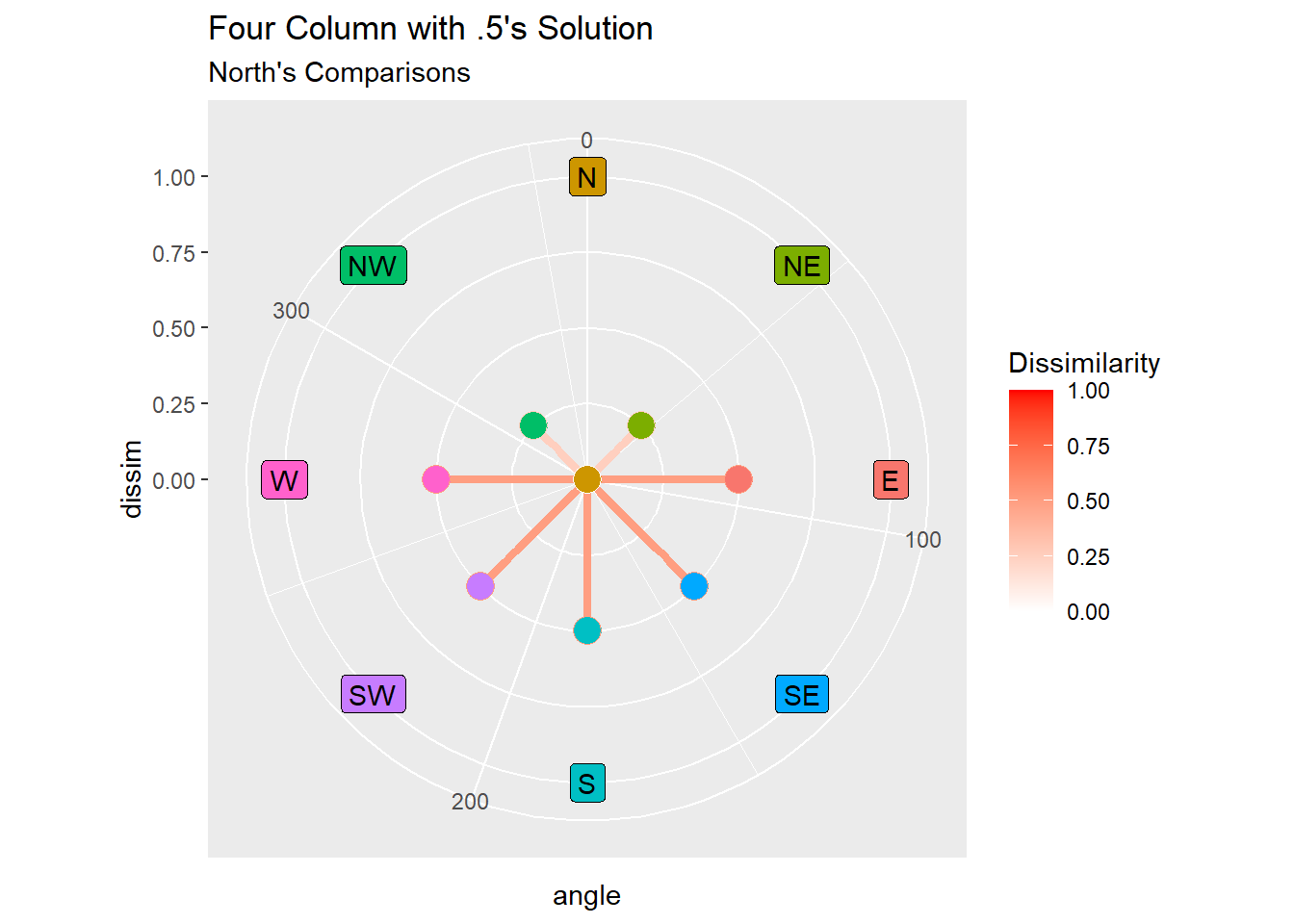
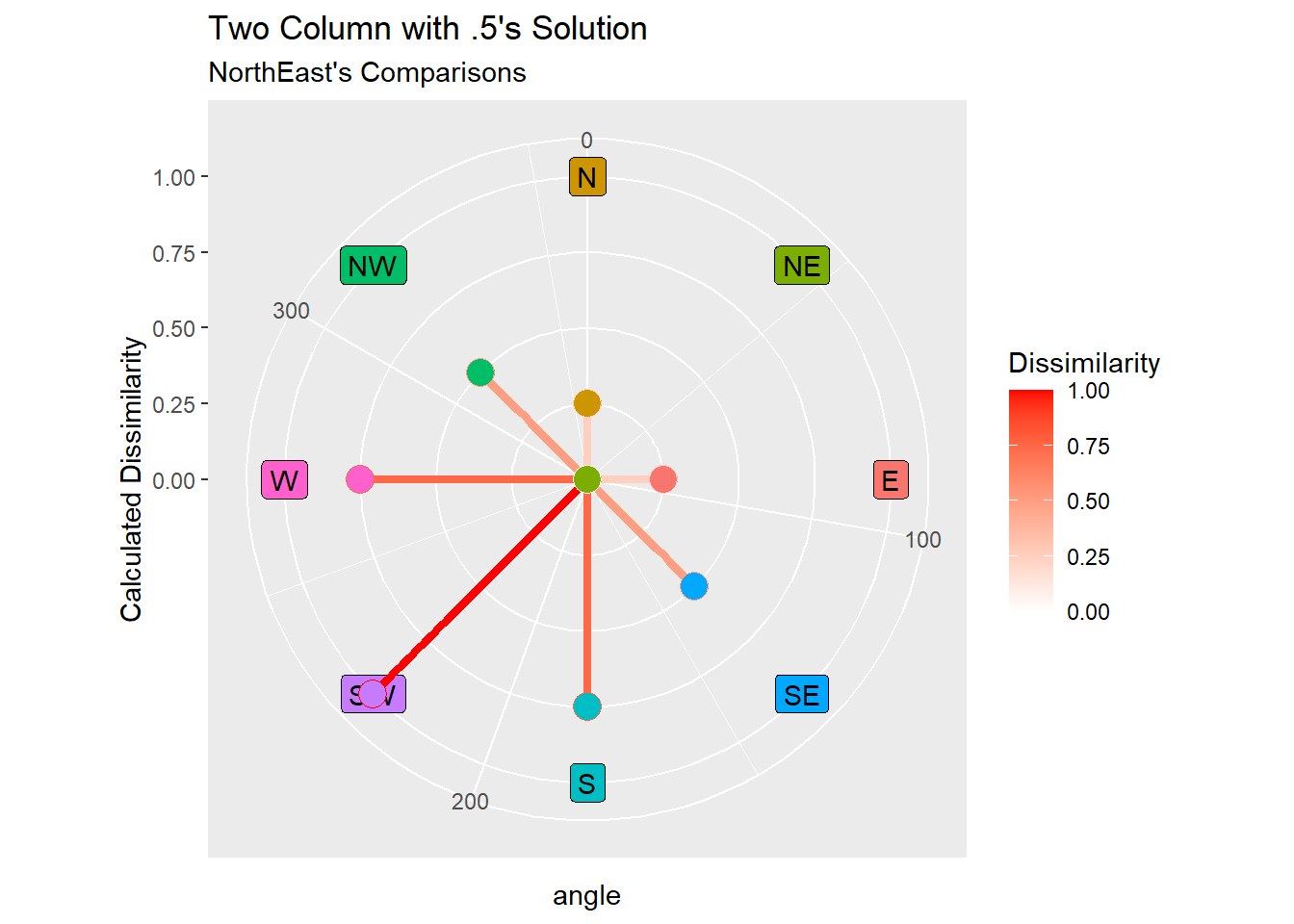
Four columns with halfs?
I thought maybe the issue was that ‘Northeast’ is kind just half North and half East. I realize now how silly that is, but I replicated the same process here.
FourColHalf<-data.frame(row.names =c("N", "NE", "E", "SE", "S", "SW","W","NW"), N =c(1,0.5,0,0,0,0,0,0.5), S =c(0,0,0,0.5,1,0.5,0,0), W =c(0,0,0,0,0,0.5,1,0.5), E =c(0,0.5,1,0.5,0,0,0,0))FourColHalf
     N   S   W   E
N  1.0 0.0 0.0 0.0
NE 0.5 0.0 0.0 0.5
E  0.0 0.0 0.0 1.0
SE 0.0 0.5 0.0 0.5
S  0.0 1.0 0.0 0.0
SW 0.0 0.5 0.5 0.0
W  0.0 0.0 1.0 0.0
NW 0.5 0.0 0.5 0.0
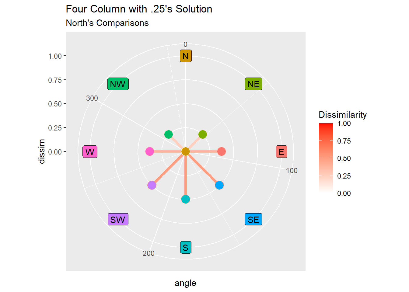
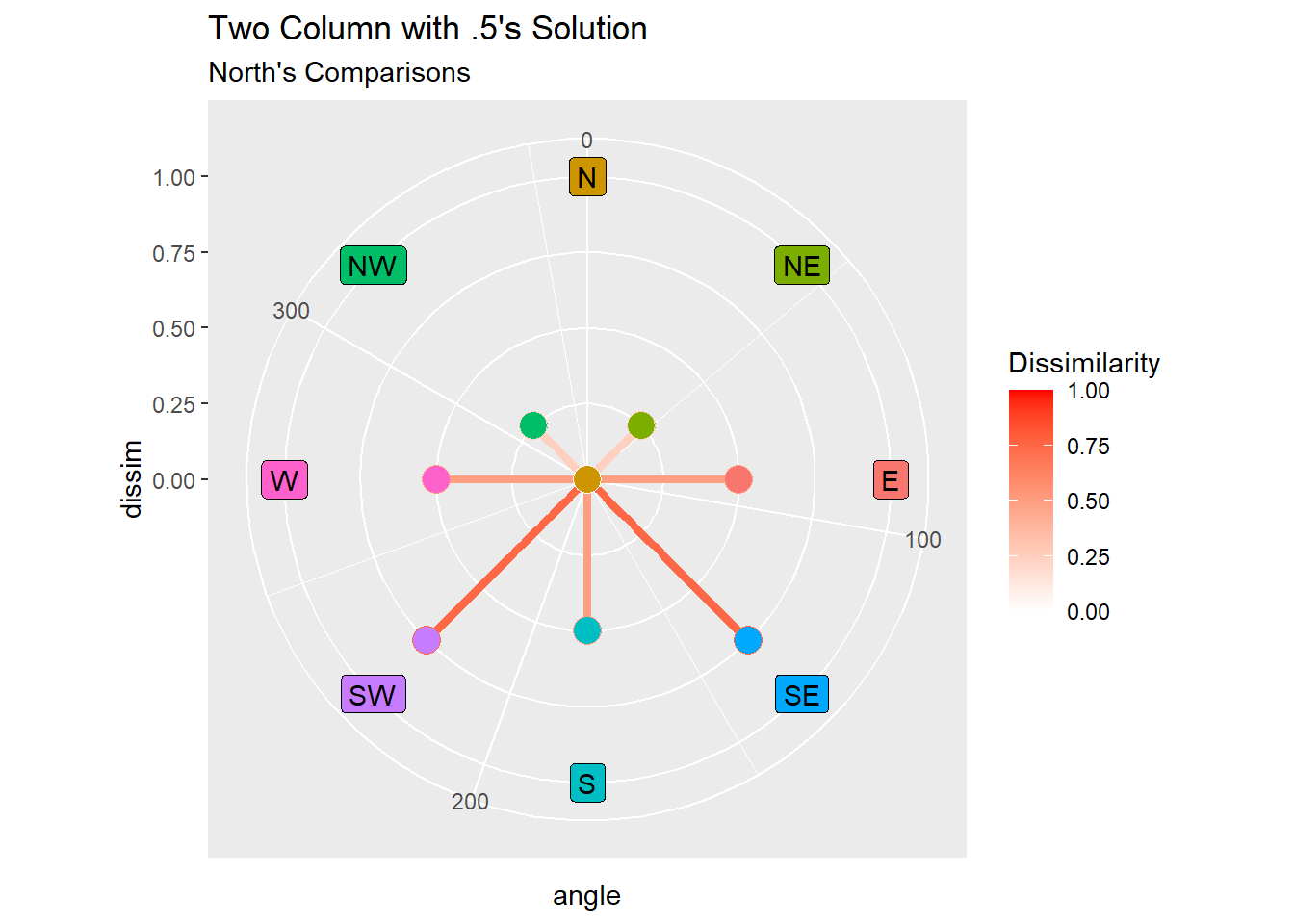
ggplot(data = FourHalfNorth, aes(x = angle, y = dissim, color = dissim, fill = direction))+coord_polar(clip ="off")+scale_x_continuous(limits =c(0,360))+scale_y_continuous(limits =c(0,1))+geom_label(aes(label = direction, x = angle, y =1), color ="black")+geom_segment(aes(y =0, yend = dissim), size =1.5)+geom_point(size=5, shape =21)+scale_color_gradient2( high="red", limits =c(0, 1), name ="Dissimilarity")+labs(title ="Four Column with .5's Solution", subtitle ="North's Comparisons")+scale_fill_discrete(guide ="none")
Warning: Using `size` aesthetic for lines was deprecated in ggplot2 3.4.0.
ℹ Please use `linewidth` instead.
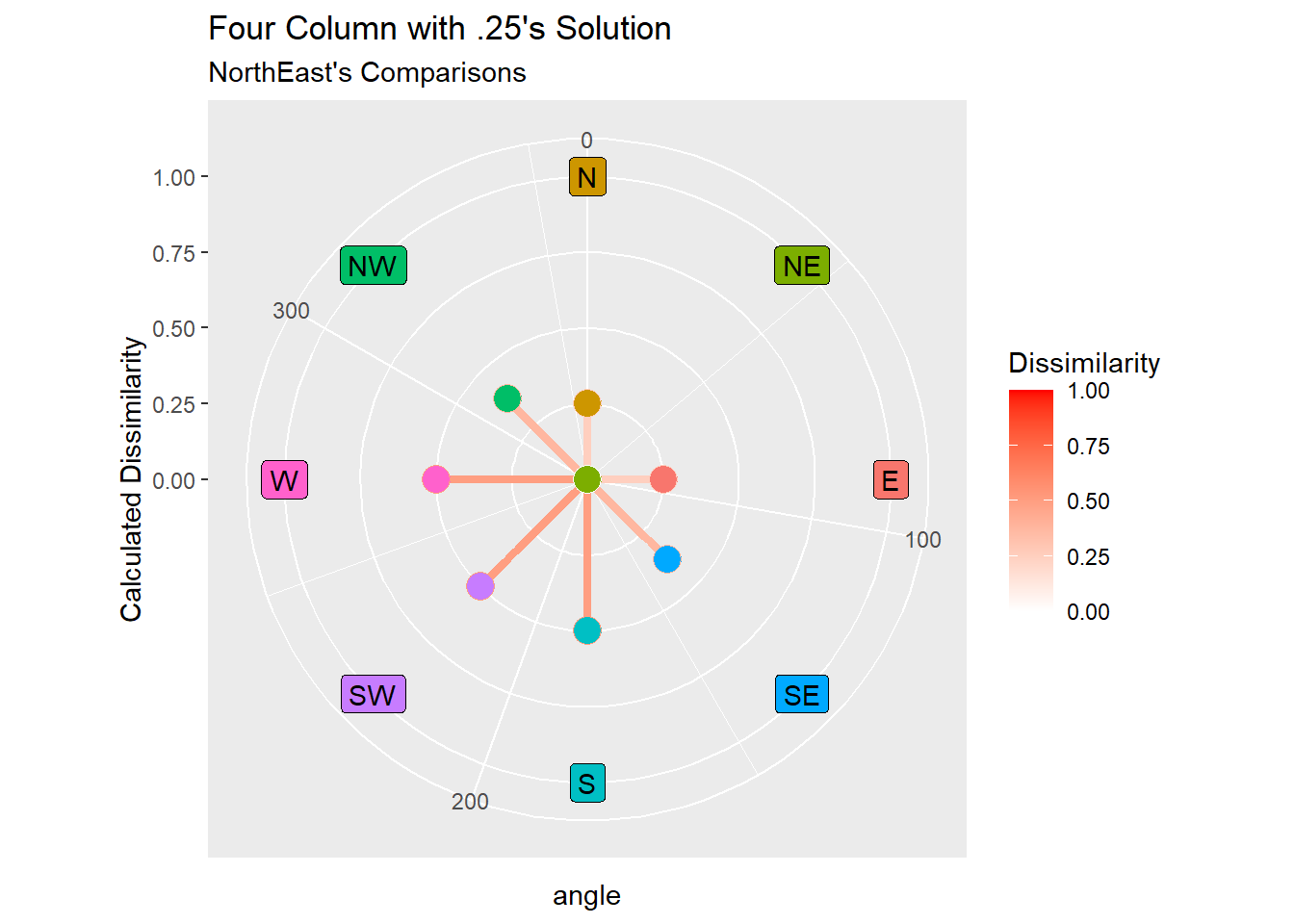
ggplot(data = FourHalfNE, aes(x = angle, y = dissim, color = dissim, fill = direction))+coord_polar(clip ="off")+scale_x_continuous(limits =c(0,360))+scale_y_continuous(limits =c(0,1))+geom_label(aes(label = direction, x = angle, y =1), color ="black")+geom_segment(aes(y =0, yend = dissim), size =1.5)+geom_point(size=5, shape =21)+scale_color_gradient2( high="red", limits =c(0, 1), name ="Dissimilarity")+labs(title ="Four Column with .5's Solution", subtitle ="NorthEast's Comparisons", y ="Calculated Dissimilarity")+scale_fill_discrete(guide ="none")
It is kind of impressive how much worse this is. Now things aren’t dissimilar enough in addition to Northeast’s having a different shape!
Four column weird
Well, okay, this is even harder to defend. I tried to make each column a spectrum. Like, with N_S being 1 to 0 how north to south a direction is. North would be a 1 there, .75 on the NW_SE and NE_SW scales, and neither East nor West (0.5). Let’s see how well this did not work!
N NW W SW S SE E NE
N 0.25 0.50 0.75 0.50 0.75 0.50 0.25
NW 0.25 0.25 0.50 0.75 1.00 0.75 0.50
W 0.50 0.25 0.25 0.50 0.75 0.50 0.75
SW 0.75 0.50 0.25 0.25 0.50 0.75 1.00
S 0.50 0.75 0.50 0.25 0.25 0.50 0.75
SE 0.75 1.00 0.75 0.50 0.25 0.25 0.50
E 0.50 0.75 0.50 0.75 0.50 0.25 0.25
NE 0.25 0.50 0.75 1.00 0.75 0.50 0.25
dist(FourCol, method ="binary")
N NE E SE S SW W
NE 0.5000000
E 1.0000000 0.5000000
SE 1.0000000 0.6666667 0.5000000
S 1.0000000 1.0000000 1.0000000 0.5000000
SW 1.0000000 1.0000000 1.0000000 0.6666667 0.5000000
W 1.0000000 1.0000000 1.0000000 1.0000000 1.0000000 0.5000000
NW 0.5000000 0.6666667 1.0000000 1.0000000 1.0000000 0.6666667 0.5000000
N_S NW_SE E_W
N 1.00 0.75 0.50
NW 0.75 1.00 0.25
W 0.50 0.75 0.00
SW 0.25 0.50 0.25
S 0.00 0.25 0.50
SE 0.25 0.00 0.75
E 0.50 0.25 1.00
NE 0.75 0.50 0.75
rowSums(FourColWeird)
  N  NW   W  SW   S  SE   E  NE
3.0 2.5 1.5 1.0 1.0 1.5 2.5 3.0
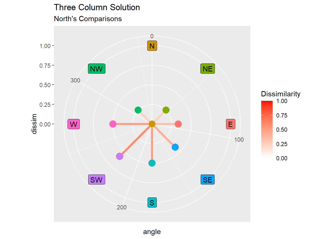
ThreeDis<-vegdist(ThreeCol, method ='gower')ThreeDis #not even close
           N        NW         W        SW         S        SE         E
NW 0.2500000
W  0.3333333 0.2500000
SW 0.4166667 0.3333333 0.2500000
S  0.5000000 0.5833333 0.5000000 0.2500000
SE 0.5833333 0.6666667 0.5833333 0.3333333 0.2500000
E  0.5000000 0.5833333 0.5000000 0.4166667 0.3333333 0.2500000
NE 0.2500000 0.3333333 0.4166667 0.3333333 0.4166667 0.3333333 0.2500000
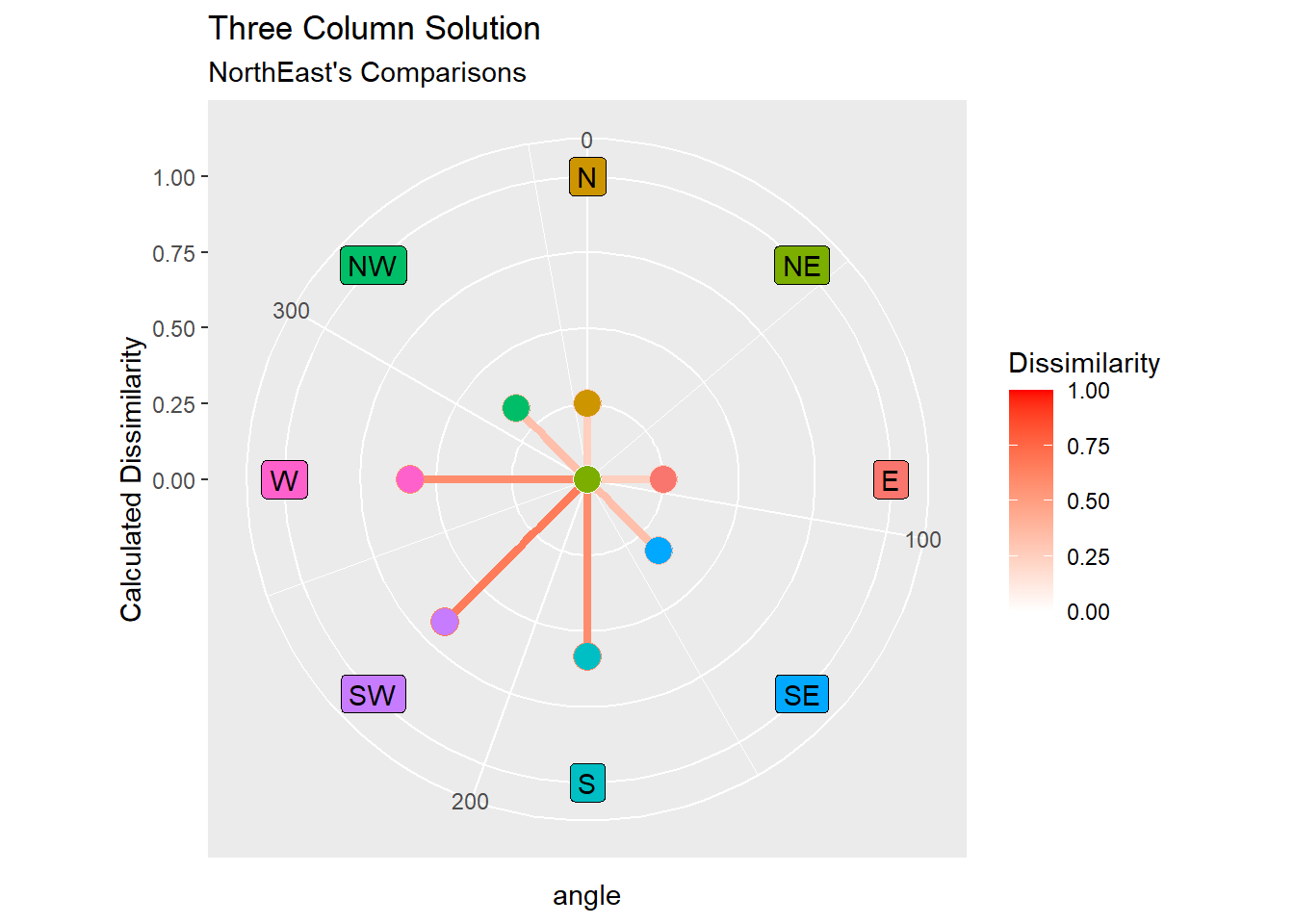
ThreeColNorth<-cbind(plotsetup, dissim =as.matrix(ThreeDis)[,1])ThreeColNE<-cbind(plotsetup, dissim =as.matrix(ThreeDis)[,2])ggplot(data = ThreeColNorth, aes(x = angle, y = dissim, color = dissim, fill = direction))+coord_polar(clip ="off")+scale_x_continuous(limits =c(0,360))+scale_y_continuous(limits =c(0,1))+geom_label(aes(label = direction, x = angle, y =1), color ="black")+geom_segment(aes(y =0, yend = dissim), size =1.5)+geom_point(size=5, shape =21)+scale_color_gradient2( high="red", limits =c(0, 1), name ="Dissimilarity")+labs(title ="Three Column Solution", subtitle ="North's Comparisons")+scale_fill_discrete(guide ="none")
ggplot(data = ThreeColNE, aes(x = angle, y = dissim, color = dissim, fill = direction))+coord_polar(clip ="off")+scale_x_continuous(limits =c(0,360))+scale_y_continuous(limits =c(0,1))+geom_label(aes(label = direction, x = angle, y =1), color ="black")+geom_segment(aes(y =0, yend = dissim), size =1.5)+geom_point(size=5, shape =21)+scale_color_gradient2( high="red", limits =c(0, 1), name ="Dissimilarity")+labs(title ="Three Column Solution", subtitle ="NorthEast's Comparisons", y ="Calculated Dissimilarity")+scale_fill_discrete(guide ="none")
LOL! Just terrible. Lopsided, gross, ugly, rude.
circular
On the verge of giving up, I turned to the one place I swore I never would: geometry. Turns out that radians things from back in the day gets the job done. Shout out to the circular package!
library(circular)#just assign them their actual anglesCircle <-data.frame(row.names =c("N", "NW","W","SW", "S", "SE","E","NE"), Angle =c(0,45,90,135,180,225,270,315))Circle
   Angle
N      0
NW    45
W     90
SW   135
S    180
SE   225
E    270
NE   315
dist.circular(Circle) #just doing it raw doesn't work, btw
Warning in as.circular(x): an object is coerced to the class 'circular' using default value for the following components:
  type: 'angles'
  units: 'radians'
  template: 'none'
  modulo: 'asis'
  zero: 0
  rotation: 'counter'
conversion.circularxradians0counter2pi
     N  NW   W  SW   S  SE   E
NW NaN
W  NaN NaN
SW NaN NaN NaN
S  NaN NaN NaN NaN
SE NaN NaN NaN NaN   0
E  NaN NaN NaN NaN   0   0
NE NaN NaN NaN NaN NaN NaN NaN
Circ<-circular(Circle, rotation ="clock") #this command does something like turning it into a specirfic circular objectCirc
Circular Data:
Type = angles
Units = radians
Template = none
Modulo = asis
Zero = 0
Rotation = clock
   Angle
N      0
NW    45
W     90
SW   135
S    180
SE   225
E    270
NE   315
dist.circular(Circ) #but it is not enough!
     N  NW   W  SW   S  SE   E
NW NaN
W  NaN   0
SW NaN   0   0
S  NaN NaN NaN NaN
SE NaN NaN NaN NaN NaN
E  NaN NaN NaN NaN NaN NaN
NE NaN   0   0   0 NaN NaN NaN
Cic<-circular(Circle, units ="degrees", modulo ="2pi", rotation ="clock", template ="geographics") #I found this works. Not sure why but yeahCic
Circular Data:
Type = angles
Units = degrees
Template = geographics
Modulo = 2pi
Zero = 1.570796
Rotation = clock
   Angle
N      0
NW    45
W     90
SW   135
S    180
SE   225
E    270
NE   315
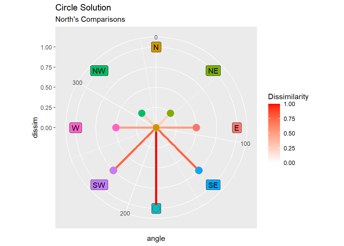
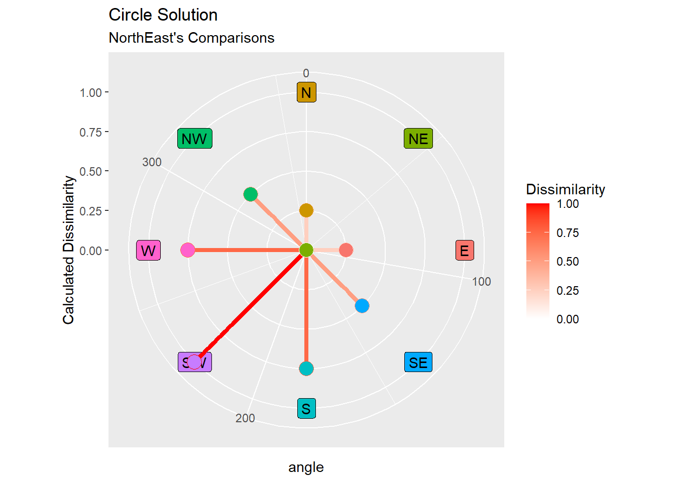
CircleDiss<-dist.circular(Cic, method ="geodesic", upper =TRUE)/pi #well this actually make the most senseCircleDiss
      N   NW    W   SW    S   SE    E   NE
N       0.25 0.50 0.75 1.00 0.75 0.50 0.25
NW 0.25      0.25 0.50 0.75 1.00 0.75 0.50
W  0.50 0.25      0.25 0.50 0.75 1.00 0.75
SW 0.75 0.50 0.25      0.25 0.50 0.75 1.00
S  1.00 0.75 0.50 0.25      0.25 0.50 0.75
SE 0.75 1.00 0.75 0.50 0.25      0.25 0.50
E  0.50 0.75 1.00 0.75 0.50 0.25      0.25
NE 0.25 0.50 0.75 1.00 0.75 0.50 0.25
rowSums(as.matrix(CircleDiss)) # AHHHH it adds up!!!!
 N NW  W SW  S SE  E NE
 4  4  4  4  4  4  4  4
CircleNorth<-cbind(plotsetup, dissim =as.matrix(CircleDiss)[,1])CircleNE<-cbind(plotsetup, dissim =as.matrix(CircleDiss)[,2])ggplot(data = CircleNorth, aes(x = angle, y = dissim, color = dissim, fill = direction))+coord_polar(clip ="off")+scale_x_continuous(limits =c(0,360))+scale_y_continuous(limits =c(0,1))+geom_label(aes(label = direction, x = angle, y =1), color ="black")+geom_segment(aes(y =0, yend = dissim), size =1.5)+geom_point(size=5, shape =21)+scale_color_gradient2( high="red", limits =c(0, 1), name ="Dissimilarity")+labs(title ="Circle Solution", subtitle ="North's Comparisons")+scale_fill_discrete(guide ="none")
ggplot(data = CircleNE, aes(x = angle, y = dissim, color = dissim, fill = direction))+coord_polar(clip ="off")+scale_x_continuous(limits =c(0,360))+scale_y_continuous(limits =c(0,1))+geom_label(aes(label = direction, x = angle, y =1), color ="black")+geom_segment(aes(y =0, yend = dissim), size =1.5)+geom_point(size=5, shape =21)+scale_color_gradient2( high="red", limits =c(0, 1), name ="Dissimilarity")+labs(title ="Circle Solution", subtitle ="NorthEast's Comparisons", y ="Calculated Dissimilarity")+scale_fill_discrete(guide ="none")
As you can see, these graphs line up and are beautiful and perfect. You can now calculate the distance between plots, geometrically with this method! This measure of distance is the same as any other dissimilarity matrix. You can actually just combine it with another dissimiliratiy matrix (like one with your other, non-circular, environmental variables) relatively easily like